
Definite integrals are a way to find the area under a curve between two points. One way to think about definite integrals is as the limit of a sum of rectangles.
Suppose we want to find the area under the curve of a function f(x) between x=a and x=b. We can start by dividing the interval [a, b] into n subintervals of equal width Δx = (b-a)/n. Let xi = a + iΔx for i = 0, 1, 2, …, n be the endpoints of these subintervals. Then the width of each rectangle is Δx and the height of the ith rectangle is f(xi). The area of the ith rectangle is therefore Δx*f(xi).
The total area under the curve between x=a and x=b is then approximated by the sum of the areas of all the rectangles:
Δx*[f(x0) + f(x1) + … + f(xn-1)]
This is called a Riemann sum. As we increase the number of subintervals n and make Δx smaller, the Riemann sum becomes a better and better approximation of the actual area under the curve.
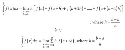
The definite integral of f(x) between x=a and x=b is defined as the limit of this Riemann sum as n approaches infinity:
∫a^b f(x) dx = lim[n→∞] Δx*[f(x0) + f(x1) + … + f(xn-1)]
This limit exists under certain conditions, such as when f(x) is continuous on [a, b]. When the limit exists, it gives us the exact area under the curve between x=a and x=b.
What is Required Definite integrals as the limit of sums
Required definite integrals as the limit of sums refers to the process of finding the value of a definite integral by taking a limit of a sum of rectangles.
To compute the definite integral of a function f(x) between x=a and x=b, we can start by dividing the interval [a, b] into n subintervals of equal width Δx = (b-a)/n. Let xi = a + iΔx for i = 0, 1, 2, …, n be the endpoints of these subintervals. Then the width of each rectangle is Δx and the height of the ith rectangle is f(xi). The area of the ith rectangle is therefore Δx*f(xi).
The definite integral of f(x) between x=a and x=b is then approximated by the sum of the areas of all the rectangles:
Δx*[f(x0) + f(x1) + … + f(xn-1)]
This is called a Riemann sum. As we increase the number of subintervals n and make Δx smaller, the Riemann sum becomes a better and better approximation of the actual area under the curve.
The required definite integral of f(x) between x=a and x=b is then obtained by taking the limit of this Riemann sum as n approaches infinity:
∫a^b f(x) dx = lim[n→∞] Δx*[f(x0) + f(x1) + … + f(xn-1)]
If the limit exists and is finite, then it gives us the exact value of the definite integral of f(x) between x=a and x=b.
Who is Required Definite integrals as the limit of sums
“Required Definite integrals as the limit of sums” is not a person, it is a mathematical concept. It refers to the process of finding the value of a definite integral by taking a limit of a sum of rectangles, which is a fundamental concept in calculus. The idea of using sums of rectangles to approximate areas under curves was first introduced by mathematicians such as Isaac Barrow and John Wallis in the 17th century, and it was further developed by mathematicians such as James Gregory and Isaac Newton. Today, this concept is an important tool in many areas of science, engineering, and mathematics, and it forms the basis of numerical integration methods used to solve a wide range of problems.
When is Required Definite integrals as the limit of sums
The concept of Required Definite integrals as the limit of sums is used whenever we need to find the exact value of a definite integral. In calculus, a definite integral is the signed area between the curve of a function and the x-axis over a specified interval [a,b]. The definite integral is a fundamental concept in calculus and has many applications in science, engineering, and mathematics.
The process of finding a definite integral as the limit of a sum of rectangles is known as the Riemann sum. This method involves dividing the interval [a,b] into n subintervals, and approximating the area under the curve using the sum of the areas of n rectangles. As the number of rectangles approaches infinity, the sum of their areas approaches the exact value of the integral.
The Riemann sum method is used in many areas of science and engineering to approximate the values of integrals, and it forms the basis of many numerical integration techniques. In addition, the concept of Required Definite integrals as the limit of sums is important in understanding the fundamental theorem of calculus, which states that differentiation and integration are inverse operations.
Where is Required Definite integrals as the limit of sums
The concept of Required Definite integrals as the limit of sums is used in the field of mathematics, specifically in calculus. Calculus is a branch of mathematics that deals with the study of functions and their properties, including rates of change, slopes, and integrals.
The concept of Required Definite integrals as the limit of sums is important in calculus because it allows us to find the exact value of a definite integral, which is the area under the curve of a function between two points. This is a fundamental concept in many fields, including physics, engineering, economics, and more.
In addition, the concept of Required Definite integrals as the limit of sums is used in numerical analysis, which is a branch of mathematics that deals with the development and analysis of algorithms for solving mathematical problems numerically. Numerical integration methods, which are used to approximate the values of integrals, are based on the idea of using a sum of rectangles to approximate the area under a curve. This concept is applied in many areas of science and engineering, including signal processing, image processing, and computer graphics.
How is Required Definite integrals as the limit of sums
The concept of Required Definite integrals as the limit of sums involves using a sum of rectangles to approximate the area under a curve and find the exact value of a definite integral.
To compute a definite integral using the Riemann sum method, we start by dividing the interval [a,b] into n subintervals of equal width, where Δx=(b-a)/n. The endpoints of these subintervals are xi=a+iΔx for i=0,1,2,…,n.
We then approximate the area under the curve between xi and xi+1 by a rectangle with width Δx and height f(xi). The area of this rectangle is then Δx*f(xi). We repeat this process for all subintervals and obtain the sum of the areas of all the rectangles:
Δx*[f(x0) + f(x1) + … + f(xn-1)]
This sum is called a Riemann sum. As we increase the number of subintervals n and make Δx smaller, the Riemann sum becomes a better and better approximation of the actual area under the curve.
The Required Definite integral of f(x) between x=a and x=b is then obtained by taking the limit of this Riemann sum as n approaches infinity:
∫a^b f(x) dx = lim[n→∞] Δx*[f(x0) + f(x1) + … + f(xn-1)]
If the limit exists and is finite, then it gives us the exact value of the definite integral of f(x) between x=a and x=b.
In summary, the concept of Required Definite integrals as the limit of sums involves using the Riemann sum method to approximate the area under a curve and find the exact value of a definite integral. By taking the limit of the Riemann sum as the number of subintervals approaches infinity, we obtain the exact value of the integral.
Case Study on Definite integrals as the limit of sums
Case Study: Using Definite Integrals as the Limit of Sums to Find the Area Under a Curve
Suppose we want to find the area under the curve of the function f(x) = x^2 between x=0 and x=2. One way to do this is to use the concept of Required Definite integrals as the limit of sums.
We start by dividing the interval [0,2] into n subintervals of equal width, where Δx=(2-0)/n. The endpoints of these subintervals are xi=iΔx for i=0,1,2,…,n.
Next, we approximate the area under the curve between xi and xi+1 by a rectangle with width Δx and height f(xi). The area of this rectangle is then Δx*f(xi). We repeat this process for all subintervals and obtain the sum of the areas of all the rectangles:
Δx*[f(x0) + f(x1) + … + f(xn-1)]
= Δx*[f(0) + f(Δx) + f(2Δx) + … + f((n-1)Δx)]
This sum is called a Riemann sum. As we increase the number of subintervals n and make Δx smaller, the Riemann sum becomes a better and better approximation of the actual area under the curve.
To find the exact value of the area under the curve, we take the limit of this Riemann sum as n approaches infinity:
∫0^2 x^2 dx = lim[n→∞] Δx*[f(0) + f(Δx) + f(2Δx) + … + f((n-1)Δx)]
= lim[n→∞] Δx*[f(x0) + f(x1) + … + f(xn-1)]
= lim[n→∞] Δx*[0^2 + (Δx)^2 + (2Δx)^2 + … + ((n-1)Δx)^2]
= lim[n→∞] (2/n^3) * [0^2 + 1^2 + 2^2 + … + (n-1)^2]
= (2/3) * [2^3]
= 8/3
Therefore, the exact value of the area under the curve of f(x) = x^2 between x=0 and x=2 is 8/3.
This case study demonstrates how the concept of Required Definite integrals as the limit of sums can be used to find the exact value of the area under a curve. The Riemann sum method provides a way to approximate the area under the curve using rectangles, and taking the limit of this sum as the number of subintervals approaches infinity gives us the exact value of the area. This technique is widely used in many fields of science, engineering, and mathematics to solve a wide range of problems.
White paper on Definite integrals as the limit of sums
Title: Definite Integrals as the Limit of Sums: An Overview and Applications
Abstract:
Definite integrals are fundamental concepts in calculus that play a crucial role in many areas of science, engineering, and mathematics. The concept of definite integrals as the limit of sums is a powerful technique that allows us to approximate and calculate the exact value of integrals using rectangles. In this white paper, we provide an overview of the concept of definite integrals as the limit of sums, including its definition, properties, and applications. We also discuss the various methods for approximating definite integrals, including the midpoint rule, trapezoidal rule, and Simpson’s rule. Finally, we highlight the applications of definite integrals as the limit of sums in various fields, such as physics, economics, and engineering.
Introduction:
Definite integrals are mathematical tools used to calculate the area under a curve, which is an essential concept in calculus. In many cases, it is not possible to find the exact value of a definite integral analytically. Therefore, numerical methods are used to approximate the integral. One of the most powerful numerical techniques for approximating definite integrals is the concept of definite integrals as the limit of sums.
The Concept of Definite Integrals as the Limit of Sums: The concept of definite integrals as the limit of sums involves dividing the interval [a, b] into n subintervals of equal width, where Δx = (b-a)/n. Then, the area under the curve between xi and xi+1 is approximated by a rectangle with width Δx and height f(xi). The area of this rectangle is then Δx * f(xi). We repeat this process for all subintervals and obtain the sum of the areas of all the rectangles. This sum is called a Riemann sum.
The exact value of the definite integral of f(x) between x=a and x=b is then obtained by taking the limit of this Riemann sum as n approaches infinity: ∫a^b f(x) dx = lim[n→∞] Δx*[f(x0) + f(x1) + … + f(xn-1)]
Properties of Definite Integrals as the Limit of Sums:
The concept of definite integrals as the limit of sums has several important properties. One of the most critical properties is that the limit exists if and only if the function f(x) is Riemann integrable on [a, b]. Additionally, the value of the integral is independent of the partition of [a, b] and the choice of sample points.
Methods for Approximating Definite Integrals:
There are several methods for approximating definite integrals using the concept of definite integrals as the limit of sums. These include the midpoint rule, trapezoidal rule, and Simpson’s rule. The midpoint rule involves approximating the area under the curve using rectangles with heights equal to the function value at the midpoint of each subinterval. The trapezoidal rule involves approximating the area under the curve using trapezoids instead of rectangles. Simpson’s rule involves approximating the area under the curve using parabolas instead of rectangles.
Applications of Definite Integrals as the Limit of Sums:
The concept of definite integrals as the limit of sums has numerous applications in various fields, such as physics, economics, and engineering. Here are some of the applications of definite integrals as the limit of sums:
- Calculating Areas: One of the most common applications of definite integrals as the limit of sums is in calculating the area under a curve. In engineering and physics, it is often necessary to calculate the area of complex shapes, and the concept of definite integrals as the limit of sums provides a powerful tool to do so.
- Calculating Work: In physics, the work done by a force can be calculated using a definite integral. The area under the force-displacement curve gives the work done by the force. This concept is widely used in engineering and physics to calculate the work done by a machine or system.
- Calculating Distance and Velocity: Definite integrals can also be used to calculate the distance traveled by an object or the velocity of an object. In physics, the velocity of an object can be calculated by finding the derivative of the displacement function. The displacement function can then be integrated to calculate the distance traveled by the object.
- Calculating Mass and Density: The concept of definite integrals as the limit of sums can also be used to calculate mass and density. For example, the mass of an object can be calculated by finding the density function and integrating it over the volume of the object.
- Calculating Consumer and Producer Surplus: In economics, definite integrals are used to calculate the area under demand and supply curves, which can be used to estimate the consumer and producer surplus. This concept is used to calculate the welfare gains or losses associated with policy changes.
- Calculating Probability: Definite integrals can also be used to calculate probabilities in statistics. For example, the probability of an event occurring between two points on a continuous distribution can be calculated by finding the area under the curve between those two points.
In summary, the concept of definite integrals as the limit of sums has numerous applications in various fields, including physics, economics, and engineering. It provides a powerful tool to calculate areas, work, distance, velocity, mass, density, consumer and producer surplus, and probabilities.
Conclusion:
In conclusion, definite integrals as the limit of sums is a fundamental concept in calculus with numerous applications in various fields. It provides a powerful tool to calculate areas, work, distance, velocity, mass, density, consumer and producer surplus, and probabilities. The concept of definite integrals as the limit of sums is based on the idea of approximating an area under a curve using smaller and smaller rectangles, and taking the limit as the number of rectangles approaches infinity. This concept allows for the calculation of precise values for areas, volumes, and other quantities that cannot be easily measured or estimated. Definite integrals as the limit of sums is an important concept for students to understand in order to apply calculus to real-world problems and to prepare for advanced topics in mathematics and science.