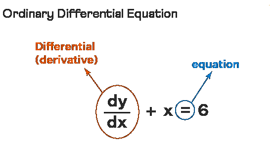
Ordinary differential equations (ODEs) describe the relationships between a function and its derivatives with respect to a single independent variable. There are several ways to form ODEs, but some of the most common are:

1. Physical laws: Many physical phenomena can be modeled using ODEs. For example, the motion of a simple pendulum can be described by the differential equation y” + (g/L)sin(y) = 0, where y is the angle of the pendulum, g is the acceleration due to gravity, and L is the length of the pendulum.
2. Mathematical models: ODEs are also commonly used to model mathematical processes, such as population growth or chemical reactions. For example, the logistic equation, which describes population growth with a carrying capacity, is given by y’ = ky(1 – y/M), where y is the population, k is a constant related to the birth and death rates, and M is the carrying capacity.
3. Empirical data: Sometimes, ODEs can be derived from empirical data. For example, the Lotka-Volterra equations, which describe the dynamics of predator-prey interactions, were originally derived from observations of real-world ecosystems.
4. Approximations: ODEs can also be formed by approximating more complicated functions. For example, the Taylor series expansion of a function can be used to derive an ODE that approximates the function near a particular point.

In general, the formation of ODEs requires an understanding of the underlying physical or mathematical principles that govern the system being studied. It may also require some creativity and mathematical skill to translate those principles into a differential equation.

What is Required Formation of ordinary differential equations

To form an ordinary differential equation (ODE), certain information is required. The information needed depends on the problem being studied and the type of ODE being formed. In general, the following information is required:

1. The dependent variable: This is the variable that is being studied and is a function of the independent variable. For example, in the case of population growth, the dependent variable is the population size.
2. The independent variable: This is the variable with respect to which the derivative of the dependent variable is taken. It could be time, distance, or any other variable that is appropriate for the problem being studied.
3. The initial or boundary conditions: These are the conditions that specify the value of the dependent variable at a particular value of the independent variable. For example, in the case of a simple pendulum, the initial condition could be the initial angle of the pendulum and its initial velocity.
4. The relationship between the dependent variable and its derivatives: This is the key information required to form the ODE. It could be based on physical laws, mathematical models, empirical data, or approximations, as discussed in the previous answer.

Once this information is obtained, it can be used to form the ODE. The ODE can then be solved using various techniques to obtain a solution that describes the behavior of the dependent variable as a function of the independent variable. The solution can then be used to make predictions or analyze the behavior of the system being studied.

Who is Required Formation of ordinary differential equations

The formation of ordinary differential equations (ODEs) is required by a variety of professionals and researchers in fields such as mathematics, physics, engineering, biology, and chemistry. Some specific examples of individuals who may require the formation of ODEs include:

1. Mathematicians: Mathematicians may form ODEs to study the behavior of functions and their derivatives, or to develop mathematical theories and methods for solving ODEs.
2. Physicists and engineers: Physicists and engineers often use ODEs to model physical phenomena such as the motion of particles or the behavior of fluids. These models can be used to make predictions, optimize designs, or analyze experimental data.
3. Biologists: Biologists may use ODEs to model biological systems such as population growth, disease spread, or cellular dynamics. These models can help predict the behavior of the system being studied and inform experimental design.
4. Chemists: Chemists may use ODEs to model chemical reactions and kinetics. These models can help predict the rate of reaction, the formation of products, and inform experimental design.

In general, the formation of ODEs is required by anyone who wants to model the behavior of a system as a function of time or another independent variable, and make predictions or analyze the behavior of that system.

When is Required Formation of ordinary differential equations

The formation of ordinary differential equations (ODEs) is required in a wide range of situations, whenever there is a need to model the behavior of a system as a function of an independent variable. Some common situations where the formation of ODEs is required include:

1. Physical systems: ODEs are commonly used to model physical systems, such as the motion of objects, the behavior of fluids, or the dynamics of electromagnetic fields.
2. Biological systems: ODEs are used to model biological systems, such as population growth, disease spread, or the dynamics of gene expression.
3. Chemical reactions: ODEs are used to model chemical reactions, including the kinetics of reactions and the behavior of reacting systems.
4. Engineering systems: ODEs are used in engineering to model a wide range of systems, such as the behavior of electrical circuits, the dynamics of control systems, or the behavior of mechanical systems.
5. Economic systems: ODEs are used to model economic systems, such as supply and demand or the dynamics of financial markets.

In general, the formation of ODEs is required whenever there is a need to understand and predict the behavior of a system over time or with respect to another independent variable. This includes a wide range of applications across many fields of study.

Where is Required Formation of ordinary differential equations

The formation of ordinary differential equations (ODEs) is required in a variety of settings, including:

1. Research institutions: Researchers in fields such as mathematics, physics, engineering, biology, chemistry, and economics may form ODEs as part of their work to model and analyze systems.
2. Universities and colleges: ODEs are commonly taught as part of undergraduate and graduate level courses in mathematics, physics, engineering, and other fields.
3. Industrial and commercial settings: ODEs are used in industries such as aerospace, automotive, and chemical manufacturing to model and optimize processes and systems.
4. Government agencies: ODEs may be used by government agencies such as the Environmental Protection Agency or the National Institutes of Health to model and analyze systems related to public health or the environment.
5. Non-profit organizations: ODEs may be used by non-profit organizations involved in environmental advocacy, public health, or social justice to model and analyze systems related to their work.

In general, the formation of ODEs is required wherever there is a need to model and analyze the behavior of a system over time or with respect to another independent variable. This can occur in a wide range of settings, including academic research, industrial processes, and government policy-making.

How is Required Formation of ordinary differential equations

The formation of ordinary differential equations (ODEs) involves several steps, which may vary depending on the problem being studied and the type of ODE being formed. Here are some general steps that are typically followed:

1. Identify the dependent and independent variables: Determine which variable represents the quantity being studied (the dependent variable) and which variable represents the independent variable with respect to which the derivative is taken.
2. Formulate the problem: Write down the mathematical relationship between the dependent variable and its derivatives, using physical laws, empirical data, mathematical models, or other sources of information.
3. State the initial or boundary conditions: Specify the value of the dependent variable at a particular value of the independent variable, either as an initial condition (for a first-order ODE) or as a set of boundary conditions (for a higher-order ODE).
4. Choose an appropriate method for solving the ODE: Depending on the problem being studied, different methods may be used to solve the ODE, such as separation of variables, integrating factors, or numerical methods.
5. Solve the ODE and interpret the solution: Use the chosen method to solve the ODE and obtain a solution that describes the behavior of the dependent variable as a function of the independent variable. Interpret the solution in the context of the problem being studied, making predictions or analyzing the behavior of the system.
6. Validate the solution: Check the solution against physical constraints or other sources of information, such as experimental data or known theoretical results.

In summary, the formation of ODEs involves identifying the variables, formulating the problem, stating the initial or boundary conditions, choosing an appropriate method for solving the ODE, solving the ODE and interpreting the solution, and validating the solution.

Case Study on Formation of ordinary differential equations

One example of the formation of ordinary differential equations (ODEs) in practice is the modeling of population growth. Let’s consider a case study of how ODEs can be used to model and analyze the growth of a population over time.

Problem statement: A population of animals is introduced into a new habitat. We want to model the growth of the population over time and analyze how different factors affect the growth rate.

Step 1: Identify the dependent and independent variables. In this case, the dependent variable is the population size, denoted by P. The independent variable is time, denoted by t.

Step 2: Formulate the problem. The rate of change of the population size is proportional to the size of the population itself, as well as to other factors such as birth rate, death rate, migration, and predation. We can formulate this relationship as follows:

dP/dt = rP(1 – P/K)

where r is the intrinsic growth rate of the population, K is the carrying capacity of the habitat (i.e., the maximum population size that the habitat can sustain), and the term (1 – P/K) represents the effect of density-dependent factors on the growth rate.

Step 3: State the initial or boundary conditions. We need to specify the initial population size, P(0), at the beginning of the simulation.

Step 4: Choose an appropriate method for solving the ODE. In this case, the ODE can be solved analytically using separation of variables, or numerically using numerical integration methods such as Euler’s method or the Runge-Kutta method.

Step 5: Solve the ODE and interpret the solution. Solving the ODE gives us a function that describes the population size as a function of time, P(t). We can use this function to make predictions about the growth of the population under different conditions, such as different initial populations, different intrinsic growth rates, or different carrying capacities. We can also analyze the behavior of the system, such as the existence of equilibrium points, stability properties, or bifurcations.

Step 6: Validate the solution. We can validate the solution by comparing the predicted population size with actual data or with known theoretical results. We can also check the behavior of the solution against physical constraints, such as non-negativity or boundedness of the population size.

In conclusion, the formation of ODEs is a powerful tool for modeling and analyzing complex systems, such as population growth. By following a systematic approach to formulating and solving ODEs, we can gain insights into the behavior of the system and make predictions that can be used for practical purposes.

White paper on Formation of ordinary differential equations

Introduction:

Ordinary differential equations (ODEs) are mathematical models that describe the behavior of a system in terms of the rate of change of one or more dependent variables with respect to an independent variable, usually time. ODEs are widely used in many areas of science and engineering to model and analyze complex phenomena, such as population dynamics, chemical reactions, mechanical systems, and electrical circuits. This white paper provides an overview of the formation of ordinary differential equations and their applications, with a focus on their mathematical properties and computational methods.

Mathematical Formulation of ODEs:

The general form of a first-order ODE is:

dy/dx = f(x, y)

where y is the dependent variable, x is the independent variable, and f(x, y) is a function that describes the rate of change of y with respect to x. The solution of this ODE is a function y(x) that satisfies the differential equation and any given initial or boundary conditions. Higher-order ODEs involve multiple derivatives of the dependent variable with respect to the independent variable and can be written in the form:

d^ny/dx^n = f(x, y, y’, y”, …, y^(n-1))

where n is the order of the ODE, y’ denotes the first derivative of y, y” denotes the second derivative, and so on.

Methods for Solving ODEs:

ODEs can be solved analytically or numerically, depending on the complexity of the equation and the availability of closed-form solutions. Analytical methods involve finding a solution in the form of an explicit or implicit function of the independent variable, using techniques such as separation of variables, integrating factors, or power series. Numerical methods involve approximating the solution of the ODE using iterative algorithms that discretize the independent variable and approximate the derivatives of the dependent variable. Examples of numerical methods include Euler’s method, the Runge-Kutta method, and the finite difference method.

Applications of ODEs:

ODEs are used in a wide range of applications, including:

• Population dynamics: modeling the growth and interaction of populations of organisms, such as animals, plants, or microorganisms.
• Chemical reactions: modeling the kinetics of chemical reactions, such as the rate of production or consumption of reactants and products over time.
• Mechanical systems: modeling the motion and forces of mechanical systems, such as vehicles, machines, or structures.
• Electrical circuits: modeling the behavior of electrical circuits, such as the flow of current, voltage, and power over time.
• Epidemiology: modeling the spread of infectious diseases and the effects of interventions such as vaccination or quarantine.

Conclusion:

ODEs are a powerful tool for modeling and analyzing complex systems in science and engineering. The formation of ODEs involves identifying the dependent and independent variables, formulating the mathematical relationship between them, stating the initial or boundary conditions, choosing an appropriate method for solving the ODE, solving the ODE and interpreting the solution, and validating the solution against physical constraints or experimental data. ODEs can be solved analytically or numerically, depending on the complexity of the equation and the availability of closed-form solutions. Numerical methods offer a versatile and efficient way to approximate the solution of ODEs, but require careful consideration of the accuracy and stability of the algorithms.