Nearest neighbors is a machine learning algorithm that is commonly used for classification and regression tasks. It works by finding the training examples in the training set that are closest to a given input example and using those examples to make a prediction.

In the context of clustering, nearest neighbors refers to a method of grouping similar data points together based on their proximity to one another. This method is often used in unsupervised learning tasks where the goal is to identify natural groupings within a dataset.

Overall, nearest neighbors is a simple and effective algorithm that can be used in a wide range of machine learning applications.

What is Required Nearest neighbours Solid State

In solid-state physics, the term “nearest neighbors” refers to the atoms that are closest in proximity to a given atom in a crystal lattice. This concept is important because the behavior of atoms in a solid can be strongly influenced by their nearest neighbors.

For example, in the study of magnetic materials, the magnetic properties of an atom can be affected by the orientation of its nearest neighbors’ spins. Similarly, in the study of semiconductors, the electrical conductivity of a material can be influenced by the arrangement of its nearest neighbor atoms.

Understanding the arrangement of nearest neighbors in a solid is therefore crucial for predicting and understanding the properties of materials, and it is a key concept in the field of solid-state physics.

Nearest neighbor search

Closest neighbor search (NNS), as a type of vicinity search, is the improvement issue of finding the point in a given set that is nearest (or generally like) a given point. Closeness is normally communicated as far as a divergence capability: the less comparable the items, the bigger the capability values.

Officially, the closest neighbor (NN) search issue is characterized as follows: given a set S of focuses in a space M and a question point q ∈ M, track down the nearest direct in S toward q. Donald Knuth in vol. 3 of The Specialty of PC Programming (1973) called it the mailing station issue, alluding to a use of relegating to a home the closest mailing station. An immediate speculation of this issue is a k-NN search, where we really want to track down the k nearest focuses.

Most usually M is a measurement space and difference is communicated as a distance metric, which is symmetric and fulfills the triangle imbalance. Considerably more normal, M is taken to be the d-layered vector space where uniqueness is estimated utilizing the Euclidean distance, Manhattan distance or other distance metric. Notwithstanding, the disparity capability can be erratic. One model is topsy-turvy Bregman disparity, for which the triangle imbalance doesn’t hold.

k-nearest neighbors algorithm

In measurements, the k-closest neighbors calculation (k-NN) is a non-parametric regulated learning strategy previously created by Evelyn Fix and Joseph Hodges in 1951, and later extended by Thomas Cover. It is utilized for grouping and relapse. In the two cases, the info comprises of the k nearest preparing models in an informational index. The result relies upon whether k-NN is utilized for characterization or relapse:

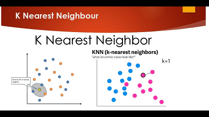
In k-NN characterization, the result is a class enrollment. An item is characterized by a majority vote of its neighbors, with the item being doled out to the class generally normal among its k closest neighbors (k is a positive number, ordinarily little). On the off chance that k = 1, the article is basically alloted to the class of that solitary closest neighbor.
In k-NN relapse, the result is the property estimation for the item. This worth is the normal of the upsides of k closest neighbors. In the event that k = 1, the result is just doled out to the worth of that solitary closest neighbor.
k-NN is a sort of characterization where the capability is just approximated locally and all calculation is conceded until capability assessment. Since this calculation depends on distance for grouping, assuming the elements address different actual units or come in boundlessly various scales then normalizing the preparation information can further develop its precision emphatically.

Both for characterization and relapse, a helpful method can be to relegate loads to the commitments of the neighbors, so that the closer neighbors offer more to the normal than the more far off ones. For instance, a typical weighting plan comprises in providing each neighbor with a load of 1/d, where d is the distance to the neighbor.

The neighbors are taken from a bunch of items for which the class (for k-NN grouping) or the item property estimation (for k-NN relapse) is known. This can be considered the preparation set for the calculation, however no express preparation step is required.

A characteristic of the k-NN calculation is that it is delicate to the nearby design of the information.

Nearest neighbour algorithm

The closest neighbors calculation was one of the primary calculations used to around take care of the mobile sales rep issue. In that issue, the sales rep begins at an irregular city and over and over visits the closest city until all have been visited. The calculation rapidly yields a short visit, yet typically not the ideal one.

Nearest neighbor graph

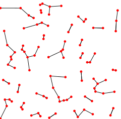
The closest neighbor diagram (NNG) is a coordinated chart characterized for a bunch of focuses in a measurement space, like the Euclidean distance in the plane. The NNG has a vertex for each point, and a guided edge from p to q at whatever point q is a closest neighbor of p, a point whose separation from p is least among every one of the given focuses other than p itself.

In many purposes of these diagrams, the headings of the edges are overlooked and the NNG is characterized rather as an undirected chart. In any case, the closest neighbor connection is definitely not a symmetric one, i.e., p from the definition isn’t really a closest neighbor for q. In hypothetical conversations of calculations a sort of broad position is frequently expected, to be specific, the closest (k-closest) neighbor is novel for each item. In executions of the calculations it is important to remember that this isn’t generally the situation. For circumstances in which it is important to make the closest neighbor for each item special, the set P might be recorded and on account of a bind the article with, e.g., the biggest list might be taken as the closest neighbor.

The k-closest neighbor diagram (k-NNG) is a chart where two vertices p and q are associated by an edge, in the event that the distance among p and q is among the k-th littlest good ways from p to different items from P. The NNG is a unique instance of the k-NNG, in particular it is the 1-NNG. k-NNGs comply with a separator hypothesis: they can be parceled into two subgraphs of at most n(d + 1)/(d + 2) vertices each by the expulsion of O(k1/dn1 − 1/d) focuses.

Another variety is the farthest neighbor diagram (FNG), in which each point is associated by an edge to the farthest point from it, rather than the closest point.

NNGs for focuses in the plane as well as in multi-layered spaces track down applications, e.g., in information pressure, movement arranging, and offices area. In measurable examination, the closest neighbor chain calculation in view of following ways in this diagram can be utilized to rapidly track down various leveled clusterings. Closest neighbor diagrams are likewise a subject of computational calculation.

The technique can be utilized to initiate a diagram on hubs with obscure network.

Nearest-neighbor interpolation

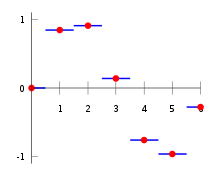
Closest neighbor addition (otherwise called proximal addition or, in certain specific circumstances, point testing) is a basic technique for multivariate introduction in at least one aspects.

Addition is the issue of approximating the worth of a capability for a non-given point in some space when given the worth of that capability in focuses around (adjoining) that point. The closest neighbor calculation chooses the worth of the closest point and doesn’t consider the benefits of adjoining focuses by any means, yielding a piecewise-steady interpolant. The calculation is exceptionally easy to carry out and is normally utilized (generally alongside mipmapping) continuously 3D delivering to choose variety values for a finished surface.

White paper on Nearest neighbours

Here is an overview of the concept of Nearest Neighbors, which can be helpful in understanding the fundamental concept behind the algorithm:

Nearest Neighbors is a machine learning algorithm that can be used for both classification and regression tasks. The algorithm works by finding the training examples in the training set that are closest to a given input example and using those examples to make a prediction.

In the context of clustering, nearest neighbors refers to a method of grouping similar data points together based on their proximity to one another. This method is often used in unsupervised learning tasks where the goal is to identify natural groupings within a dataset.

The nearest neighbors algorithm is based on the assumption that data points that are close together in the feature space have similar characteristics or belong to the same class. By finding the closest neighbors of a given data point, the algorithm can predict its class or value based on the classes or values of its neighbors.

One of the main advantages of the nearest neighbors algorithm is its simplicity and ease of implementation. It does not require any training or model building, which makes it a popular choice for small datasets or when the underlying relationships between the features and the target variable are complex and nonlinear.

However, the nearest neighbors algorithm can be computationally expensive, especially when dealing with large datasets or high-dimensional feature spaces. In addition, the algorithm is sensitive to the choice of distance metric and the number of neighbors used in the prediction, which can affect the accuracy of the results.

In summary, the nearest neighbors algorithm is a simple and effective algorithm for classification, regression, and clustering tasks that is widely used in machine learning. Its ability to identify natural groupings in a dataset and its ease of implementation make it a popular choice for many applications.