

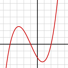
Polynomials are mathematical functions of the form:
f(x) = a_n x^n + a_{n-1} x^{n-1} + … + a_1 x + a_0
where a_n, a_{n-1}, …, a_1, a_0 are constants and n is a non-negative integer. Special polynomials are those that have particular properties or are used to solve specific problems.
Some examples of special polynomials include:
- Legendre polynomials: Legendre polynomials are a sequence of orthogonal polynomials that are solutions to the Legendre differential equation. They are commonly used in physics and engineering to solve problems involving spherical symmetry, such as the hydrogen atom.
- Chebyshev polynomials: Chebyshev polynomials are a sequence of orthogonal polynomials that have many applications in numerical analysis, including approximation theory and numerical integration. They are also used in signal processing and image analysis.
- Hermite polynomials: Hermite polynomials are a sequence of orthogonal polynomials that are solutions to the Hermite differential equation. They have applications in quantum mechanics, statistical mechanics, and electrical engineering.
- Laguerre polynomials: Laguerre polynomials are a sequence of orthogonal polynomials that are solutions to the Laguerre differential equation. They have applications in quantum mechanics, statistical mechanics, and fluid mechanics.
These special polynomials have unique properties that make them useful in various mathematical and scientific applications. They are often used to approximate other functions or to solve differential equations, and they can be computed efficiently using recursive algorithms or numerical methods.
Notation and terminology
The x occurring in a polynomial is commonly called a variable or an indeterminate. When the polynomial is considered as an expression, x is a fixed symbol which does not have any value (its value is “indeterminate”). However, when one considers the function defined by the polynomial, then x represents the argument of the function, and is therefore called a “variable”. Many authors use these two words interchangeably.
A polynomial P in the indeterminate x is commonly denoted either as P or as P(x). Formally, the name of the polynomial is P, not P(x), but the use of the functional notation P(x) dates from a time when the distinction between a polynomial and the associated function was unclear. Moreover, the functional notation is often useful for specifying, in a single phrase, a polynomial and its indeterminate. For example, “let P(x) be a polynomial” is a shorthand for “let P be a polynomial in the indeterminate x“. On the other hand, when it is not necessary to emphasize the name of the indeterminate, many formulas are much simpler and easier to read if the name(s) of the indeterminate(s) do not appear at each occurrence of the polynomial.
The ambiguity of having two notations for a single mathematical object may be formally resolved by considering the general meaning of the functional notation for polynomials. If a denotes a number, a variable, another polynomial, or, more generally, any expression, then P(a) denotes, by convention, the result of substituting a for x in P. Thus, the polynomial P defines the function

which is the polynomial function associated to P. Frequently, when using this notation, one supposes that a is a number. However, one may use it over any domain where addition and multiplication are defined (that is, any ring). In particular, if a is a polynomial then P(a) is also a polynomial.
More specifically, when a is the indeterminate x, then the image of x by this function is the polynomial P itself (substituting x for x does not change anything). In other words,

which justifies formally the existence of two notations for the same polynomial.
Degree of a polynomial
In mathematics, the degree of a polynomial is the highest of the degrees of the polynomial’s monomials (individual terms) with non-zero coefficients. The degree of a term is the sum of the exponents of the variables that appear in it, and thus is a non-negative integer. For a univariate polynomial, the degree of the polynomial is simply the highest exponent occurring in the polynomial. The term order has been used as a synonym of degree but, nowadays, may refer to several other concepts (see order of a polynomial (disambiguation)).
For example, the polynomial 

To determine the degree of a polynomial that is not in standard form, such as 

When is Required Special functions (polynomial)
Special functions (polynomials) are required when dealing with mathematical problems that involve certain types of functions that cannot be easily expressed in terms of elementary functions (such as polynomials, exponential functions, trigonometric functions, etc.). Special functions are often used to solve differential equations, partial differential equations, integral equations, and other mathematical problems that arise in physics, engineering, and other scientific fields.
For example, Legendre polynomials are used to solve problems in electrostatics, such as finding the potential and electric field around a charged spherical conductor. Chebyshev polynomials are used in numerical analysis and approximation theory, particularly in the context of Chebyshev interpolation and Chebyshev quadrature. Hermite polynomials are used in quantum mechanics to describe the wave functions of harmonic oscillators, and Laguerre polynomials are used to solve the Schrödinger equation for the hydrogen atom.
In summary, special functions (polynomials) are required when dealing with mathematical problems that cannot be solved using elementary functions alone, particularly in physics, engineering, and other scientific fields where complex mathematical models are required.
Legendre polynomials
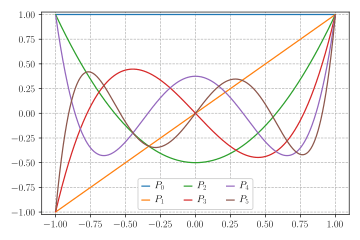
In science, Legendre polynomials, named after Adrien-Marie Legendre (1782), are an arrangement of complete and symmetrical polynomials with countless numerical properties and various applications. They can be characterized in numerous ways, and the different definitions feature various perspectives as well as recommend speculations and associations with various numerical designs and physical and mathematical applications.
Firmly connected with the Legendre polynomials are related Legendre polynomials, Legendre capabilities, Legendre elements of the subsequent kind, and related Legendre capabilities.
Hermite polynomials
In mathematics, the Hermite polynomials are a classical orthogonal polynomial sequence.
The polynomials arise in:
- signal processing as Hermitian wavelets for wavelet transform analysis
- probability, such as the Edgeworth series, as well as in connection with Brownian motion;
- combinatorics, as an example of an Appell sequence, obeying the umbral calculus;
- numerical analysis as Gaussian quadrature;
- physics, where they give rise to the eigenstates of the quantum harmonic oscillator; and they also occur in some cases of the heat equation (when the term
is present);
- systems theory in connection with nonlinear operations on Gaussian noise.
- random matrix theory in Gaussian ensembles.
Hermite polynomials were defined by Pierre-Simon Laplace in 1810, though in scarcely recognizable form, and studied in detail by Pafnuty Chebyshev in 1859. Chebyshev’s work was overlooked, and they were named later after Charles Hermite, who wrote on the polynomials in 1864, describing them as new. They were consequently not new, although Hermite was the first to define the multidimensional polynomials in his later 1865 publications.
Bernoulli polynomials
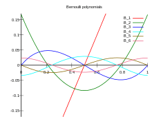
In science, the Bernoulli polynomials, named after Jacob Bernoulli, join the Bernoulli numbers and binomial coefficients. They are utilized for series development of capabilities, and with the Euler-MacLaurin equation.
These polynomials happen in the investigation of numerous extraordinary capabilities and, specifically, the Riemann zeta capability and the Hurwitz zeta capability. They are an Appell arrangement (for example a Sheffer grouping for the standard subordinate administrator). For the Bernoulli polynomials, the quantity of intersections of the x-hub in the unit stretch doesn’t go up with the degree. In the constraint of enormous degree, they approach, when suitably scaled, the sine and cosine capabilities.
A comparative arrangement of polynomials, in view of a creating capability, is the group of Euler polynomials.
Orthogonal polynomials
In science, a symmetrical polynomial succession is a group of polynomials with the end goal that any two distinct polynomials in the succession are symmetrical to one another under some internal item.
The most broadly utilized symmetrical polynomials are the old style symmetrical polynomials, comprising of the Hermite polynomials, the Laguerre polynomials and the Jacobi polynomials. The Gegenbauer polynomials structure the main class of Jacobi polynomials; they incorporate the Chebyshev polynomials, and the Legendre polynomials as extraordinary cases.
The field of symmetrical polynomials created in the late nineteenth hundred years from an investigation of proceeded with divisions by P. L. Chebyshev and was sought after by A. A. Markov and T. J. Stieltjes. They show up in a wide assortment of fields: mathematical examination (quadrature rules), likelihood hypothesis, portrayal hypothesis (of Untruth gatherings, quantum gatherings, and related objects), enumerative combinatorics, logarithmic combinatorics, numerical physical science (the hypothesis of irregular networks, integrable frameworks, and so on), and number hypothesis. A portion of the mathematicians who have dealt with symmetrical polynomials incorporate Gábor Szegő, Sergei Bernstein, Naum Akhiezer, Arthur Erdélyi, Yakov Geronimus, Wolfgang Hahn, Theodore Seio Chihara, Mourad Ismail, Waleed Al-Salam, Richard Askey, and Rehuel Lobatto.